The aim of this blog is to show that phylogenetic methods — traditionally used to reconstruct the evolutionary history of biological species — can be applied far beyond their original scope. This idea was first theorised by Dawkins in 1976 [1] and has since been demonstrated on cultural artifacts by researchers such as Julien d’Huy [2]. Here, we take it a step further and apply it to the intelligence of Large Language Models (LLMs).
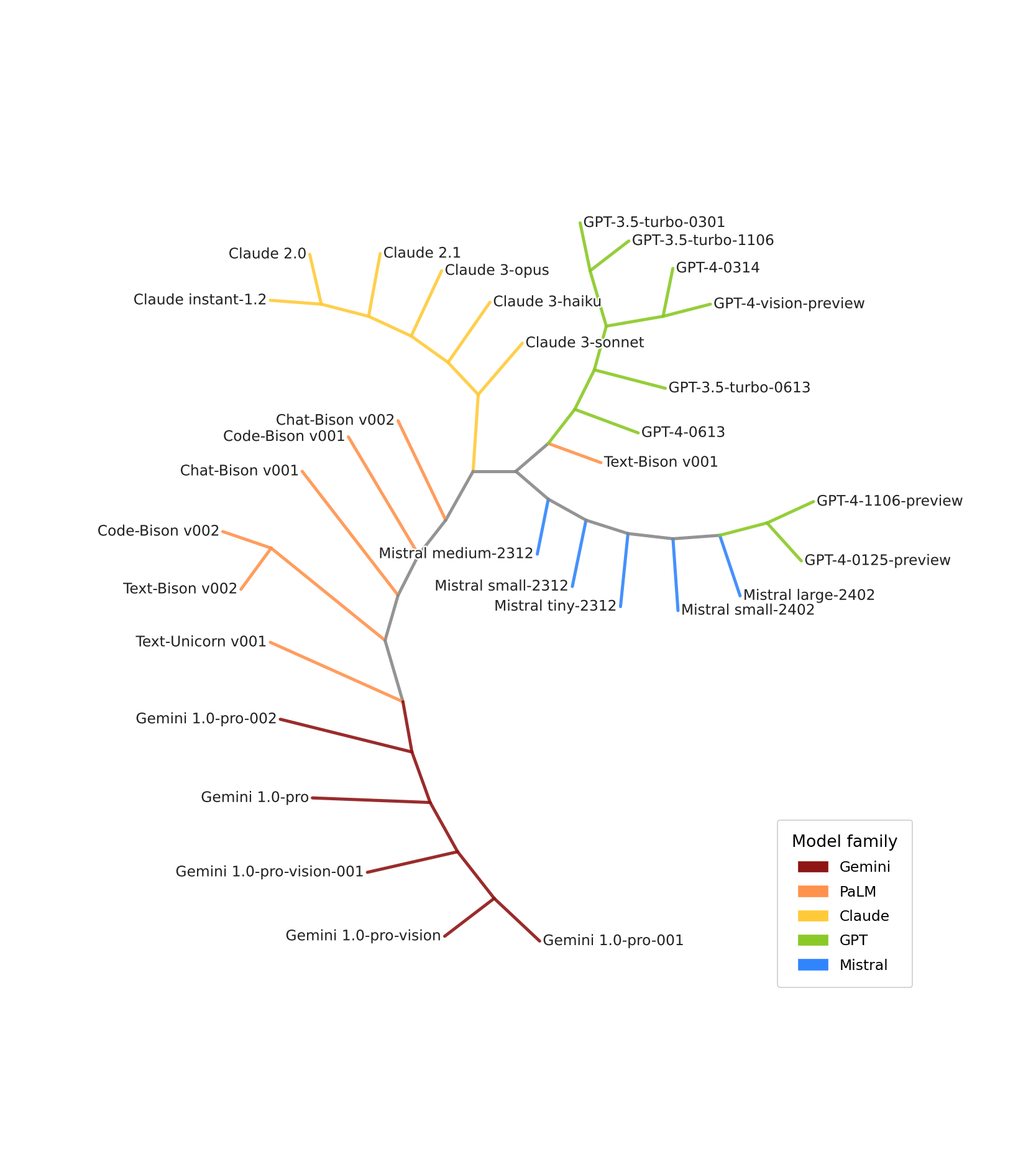
Estimated dendrogram of some LLMs from OpenAI, Anthropic, Google and Mistral.
This is a particularly timely question in a world where the number of LLMs is growing at an extraordinary pace — around 300 new models are published every day on the HuggingFace hub — and where transparency about training details is increasingly limited. Reconstructing the phylogenetic history of models in a black-box setting, without any prior information beyond interacting with them, would provide a powerful tool to map the landscape of modern AI, shed light on lineages that are not always made explicit, and inform the evaluation of AI capabilities — with potential applications to AI safety and the monitoring of emerging risks.
Part I: What is Phylogenetics ?
Phylogenetics is the study of evolutionary relationships among organisms. It involves reconstructing the evolutionary history and relatedness of different species or populations, by analyzing their characteristics and determining how they descended from common ancestors.
The main goal is to understand how different organisms are connected through evolution, typically represented in tree-like diagrams called phylogenetic trees. These trees illustrate which species share recent common ancestors, how lineages branched over time, and the sequence in which different groups evolved.
Populations of individuals that frequently reproduce with each other (sexual reproduction) or share genetic material (as bacteria often do) tend to maintain some homogeneity in their genetic data. However, when a population splits in two — think of insects in a forest divided by a fire, suddenly unable to reach one another — the genetic sharing stops, and the two groups begin evolving much more independently. When they eventually become too genetically different to reproduce with each other, they are said to have speciated: they are now two distinct species. The scenario described above — separation by geography — is known as allopatric speciation, and it’s just one of several ways speciation can occur.
With that foundation in place, let’s look at how we actually reconstruct the evolutionary history of living species from the speciations that shaped them and then how these ideas can be relevant to study the evolution of cultural artefacts and LLMs.
Methods to reconstruct phylogenetic trees in biological systems
This blog will only explore one method of reconstructing biological evolution through genetic material to give a concrete example of how such methods work.
Given a set of populations (species, animal races, communities, etc.) that we want to reconstruct the genetic evolutionary history of, we first need to select some genes common to all of them as a basis for comparison. To make this concrete, let’s imagine we want to reconstruct the evolutionary history of five cat breeds — the Persian, the Siamese, the Maine Coon, the Bengal, and the British Shorthair. One could say these are not distinct species, but the same algorithm applies to both breeds and species and it makes a great illustration example.
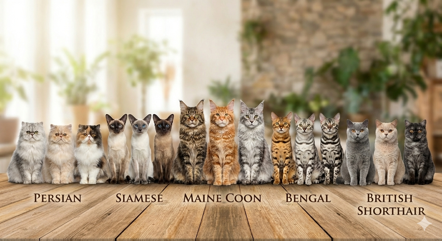 Cat breeds used for the study - image generated by Gemini for the sake of illustration in this blog.
Let’s walk through each step of the phylogenetic pipeline to understand which breeds share a recent common history and which diverged long ago.
How to select the genes ?
We need genes that varied moderately at the timescale of the study. For example, if we study a set of cat breeds, genes related to reproduction may not have varied much between breeds, offering too little variation to distinguish between them. On the other hand, genes related to fur color may offer too much variance, making all breeds appear very different from each other and the results too noisy to interpret. It is therefore important to choose genes that show moderate variance and that capture the evolutionary signal we are looking for.
To go back to our population of cats, relevant genes could be related to eye color, hair length, or overall skull morphology — traits that vary enough between breeds to be informative, but not so much as to obscure the underlying evolutionary relationships. Let’s say we select three genes for our toy study: Gene C (eye color), Gene E (ear length), and Gene S (skull morphology). Each of these genes has a small number of possible variants (alleles). For instance, Gene C might have three alleles in this toy example: blue, copper, and green; Gene E might have three: short, medium, and long; and Gene S might have two: round and elongated. To be fair, in practice these traits are not the result of a single gene or allele but usually a combination of several. For the sake of simplicity, this blog assumes a single gene per trait and uses this simplification only to illustrate the process of building a phylogenetic tree with a small and interpretable number of variables.
All the genes discussed here are functional genes, meaning they directly impact the physical attributes of the cat. In practice, many modern phylogenetic studies use DNA segments that are non-functional — not expressed, and not tied to any physical attribute. For the sake of clarity, this blog illustrates the pipeline using genes related to physical traits because it makes the process visual and easy to follow. That said, it is important to note that phylogenetic studies are grounded in the genotype of an individual (its genes) rather than its phenotype (its physical appearance), since individuals can converge on very similar appearances while having very different evolutionary histories.
Gathering genetic information
Once the genes are selected, we can gather individuals from each population of cats and measure which version of each gene they carry (called an allele). For example, in a population of Persians, we might sample 100 individuals and find that 95% carry the round skull allele and only 5% carry the elongated allele for Gene S, while in the Siamese population the split might be 15% round and 85% elongated. This is stored in a population function P(allele | gene) — the probability of finding a given allele for a given gene when sampling a random individual from that population.
Continuing with our example, here is what the population functions might look like for all five breeds across our three selected genes:
| Breed | Gene C (blue / copper / green) | Gene E (short / medium / long) | Gene S (round / elongated) |
|---|---|---|---|
| Persian | 0.05 / 0.85 / 0.10 | 0.90 / 0.10 / 0.00 | 0.95 / 0.05 |
| Siamese | 0.98 / 0.02 / 0.00 | 0.00 / 0.10 / 0.90 | 0.15 / 0.85 |
| Maine Coon | 0.05 / 0.60 / 0.35 | 0.00 / 0.15 / 0.85 | 0.30 / 0.70 |
| Bengal | 0.05 / 0.55 / 0.40 | 0.10 / 0.75 / 0.15 | 0.25 / 0.75 |
| British Shorthair | 0.03 / 0.90 / 0.07 | 0.15 / 0.80 / 0.05 | 0.85 / 0.15 |
A population function is estimated for each breed, and these distributions are then compared to measure how similar or distant the breeds are from one another.
Population comparison
Once a population function is estimated for each population studied, they are compared using a mathematical formula, which can vary between studies. For this blog we are going to use one of the most classic: Nei’s genetic distance [3], defining a similarity matrix S and a distance matrix D:
$S(P_1, P_2) = \frac{\sum_{g \in G} \sum_{a \in A_g} P_1(a|g) \cdot P_2(a|g)}{\sqrt{\left(\sum_{g \in G} \sum_{a \in A_g} P_1(a|g)^2\right) \left(\sum_{g \in G} \sum_{a \in A_g} P_2(a|g)^2\right)}}$
$D(P_1,P_2) = -\log(S(P_1,P_2))$
Where:
- $P_1$ and $P_2$ are two populations (or LLMs), seen as probability distributions of alleles given a gene
- $G$ is the set of genes considered
- $A_g$ is the set of possible alleles for gene $g$
- $S$ is the similarity matrix, bounded in $[0, 1]$
- $D$ is the distance matrix, in $[0,+\infty]$
To put it simply, the similarity formula compares the probability of seeing the same allele appear in both populations for the same gene, and normalises it by the probability of seeing that allele in each population individually. This produces a measure of how similar the two population functions are. The distance matrix D is then derived from the similarity matrix and used to plot the phylogenetic tree.
Let’s see what this similarity matrix looks like between our cat breeds:
| Persian | Siamese | Maine Coon | Bengal | British Shorthair | |
|---|---|---|---|---|---|
| Persian | 1.00 | 0.10 | 0.78 | 0.41 | 0.69 |
| Siamese | 0.10 | 1.00 | 0.35 | 0.47 | 0.22 |
| Maine Coon | 0.78 | 0.35 | 1.00 | 0.73 | 0.57 |
| Bengal | 0.41 | 0.47 | 0.73 | 1.00 | 0.77 |
| British Shorthair | 0.69 | 0.22 | 0.57 | 0.77 | 1.00 |
This matrix represents the similarity between cat breeds as seen through the lens of the selected genes. Persians and Siamese, for instance, are the most genetically distant pair in our study (0.10 similarity), while British Shorthairs and Persians appear considerably closer (0.69 similarity).
Phylogenetic tree
The concept behind plotting a phylogenetic tree is that populations which speciated recently will remain fairly similar, while populations that speciated long ago will have diverged significantly as mutations accumulate over time. This is why gene selection matters so much: genes that mutate too fast or too slowly will not efficiently capture the evolutionary history of the species studied. Several algorithms have been proposed to compute a tree from a distance matrix; the one discussed here is one of the most classic: the Neighbour-Joining technique (NJ tree) [4]. The goal is not to give a full tutorial on the NJ algorithm but to provide an overview of the approach.
The core idea is that populations which diverged most recently should be the most genetically similar. The algorithm identifies the two populations that are closest to each other relative to their distance to all other populations — not simply the two with the smallest absolute distance. These two populations are then grouped into a clade, representing their hypothetical common ancestor. Once this clade is formed, the two original populations are removed from the distance matrix and replaced by their common ancestor, whose distance to every remaining population is estimated as a weighted average of the distances from the two child populations. The matrix now has one fewer entry (n−1 instead of n). This process repeats — finding the next closest pair, grouping them, and reducing the matrix — until only two populations remain, joined at the root of the tree: the ancestor of all.
This method makes it possible to build a phylogenetic tree representing one possible version of the evolutionary history of these species, seen through the prism of the selected genes.
Back to our cats, here is the NJ tree for the five breeds:
┌──────────────────── Siamese 🐱
───┤Clade 4
│ ┌──────────────── Maine Coon 🦁
└─┤Clade 3
│ ┌──────────── Bengal 🐆
└─┤Clade 2
│ ┌──────── British Shorthair 🐈
└─┤Clade 1
└──────── Persian 🐈⬛
This is compatible with the genetic literature: British Shorthair and Persian speciated recently relative to Maine Coon or Siamese. The Bengal, however, is a special case — it is a crossbreed between Asian leopard cats and domestic European cats, meaning its evolutionary history cannot be cleanly captured by a tree structure.
This highlights a broader limitation of the approach: it rests on the assumption that evolution follows a tree-like structure, with limited interaction between lineages such as horizontal gene transfer or complex interbreeding. As domesticated animals, cats have been heavily shaped by human intervention, making their evolutionary history particularly tangled. Phylogenetic methods like the one presented here are most reliable when applied to species whose evolution more closely follows these theoretical principles.
Part 2: Theory of Evolution
We have seen how to build phylogenetic trees using a simple method. But why does it actually work? What properties of DNA make it such a reliable marker of evolutionary history, and could these properties exist in non-biological objects? This section explores the theoretical foundations of phylogenetics, which we will later use as a framework to study the evolution of cultural artifacts and language models.
DNA: the functional and archeological support for evolution
Studying past evolution revolves around finding markers of that evolution that are still accessible today. In biology, these markers are DNA mutations. When reproducing, mutations are introduced into the DNA of the offspring and may then be passed on to future generations. These mutations come in two broad flavors:
Mutations under selective pressure affect the fitness of the individual in its environment — making it more or less likely to survive and reproduce. A skin pattern that improves camouflage, or the ability to resist extreme temperatures, are classic examples. Beneficial mutations of this kind tend to spread rapidly through a population, as individuals carrying them reproduce more successfully. Harmful ones, on the other hand, are quickly eliminated: individuals who develop them tend to die before reproducing or fail to find mates, and so the mutation disappears from the gene pool. Because of this, genes that encode vital features — heart architecture, reproductive organs — show very little variation across individuals: any mutation in these genes is almost certainly harmful and gets weeded out fast.
Neutral mutations do not affect the fitness of the individual. A DNA sequence that is not expressed, or one that produces an equivalent protein, or traits like eye color that have little impact on survival or reproduction — these can accumulate freely across generations. Because they are not filtered by selection, they evolve at a much steadier and more predictable rate, making them the most useful markers for tracing evolutionary history. The further back two populations diverged, the more neutral mutations will have accumulated between them. Because neutral mutations are not filtered by selection, their accumulation is driven primarily by random chance — a process known as genetic drift. This randomness is actually what makes neutral genes such reliable evolutionary clocks: drift operates at a relatively steady rate, unlike selection which is episodic and environment-dependent.
This distinction is crucial: genes under strong selective pressure evolve slowly, while neutral genes evolve more steadily. Phylogenetics primarily relies on the latter to reconstruct the branching history of species especially for smaller time scale studies (as discussed above with cats).
This makes DNA a remarkable dual-purpose molecule: it is both the functional driver of evolution and its archeological record. In the next section, we will try to abstract away from the biology and ask what properties make DNA so well suited to this role — because those properties, as we will see, are not unique to biological objects.
What makes a good marker of evolutionary history?
Before Darwin, evolutionary studies relied primarily on phenotype — researchers attempted to deduce evolutionary relationships from the appearance of species. But individuals are extraordinarily high-dimensional objects: every feature may evolve at a different rate, and many superficial similarities turn out to be the product of convergent evolution rather than shared ancestry. Two species can look alike simply because they adapted to the same environment, not because they are closely related. As Darwin himself argued, functional characteristics — what an organism does and how it works — are far more directly tied to evolutionary history than surface appearance alone.
This is precisely what makes DNA such an effective marker. It is a compressed and universal representation of the individual: vastly smaller than a full description of the organism yet capturing the core logic that shapes it, expressed in a common biochemical language that can be compared across wildly different species. It encodes functional identity rather than superficial similarity — the underlying architecture of the organism rather than its appearance. And crucially, at least for the right choice of genes, it evolves at a moderate and relatively steady rate — not so fast that the historical signal is lost in noise, and not so slow that no variation accumulates between populations.
These three properties:
- (1) compression and universality (which implies a combinatorial encoding),
- (2) a moderate evolutionary rate,
- (3) and functional grounding,
are what makes DNA well suited to phylogenetic reconstruction. And if these are the key properties, then DNA need not be the only object that satisfies them. As we will explore in the next part, similar structures may exist far beyond biology.
The limits of tree-based models
The methodology described above still has important limitations, as the Bengal cat already illustrated. It assumes a strictly tree-like model of evolution, and therefore does not easily account for horizontal gene transfer, convergent evolution, or interbreeding between distinct lineages. In reality, evolutionary history is often more of a tangled web than a clean branching tree. It is important to keep in mind that phylogenetic trees are powerful approximations, but approximations nonetheless — and we will see this tension resurface in practice when we move beyond biology.
Part 3: Phylogenetics Beyond Biology
We have seen in the previous section that the properties of DNA which make it a particularly powerful tool for reconstructing evolutionary lineages may also be found in non-biological objects, opening the door to applying phylogenetic techniques beyond biology. This section presents several studies that do exactly this, focusing on cultural artifacts — objects created by humans that carry information about the culture of their creators and users — in order to trace their cultural evolution.
Cultural evolution
Just as biological species evolve under the pressure of their environment, cultural objects evolve under the pressure of the societies that produce and transmit them. An idea, a story, a tool, or a tradition does not remain static as it passes from person to person and generation to generation — it mutates, gets selected, and drifts, much like a genome. Some variations spread because they are more compelling, more useful, or more memorable; others disappear because they fail to resonate or survive transmission. This process, driven by human minds rather than biology, is what we call cultural evolution.
What makes cultural evolution particularly fascinating — and particularly amenable to phylogenetic analysis — is that it leaves traces. Cultural objects carry within them the marks of their history: a myth preserves echoes of the society that first told it, a tool reflects the constraints and knowledge of the civilization that built it. If we can identify the right markers of this history — the cultural equivalent of genes — we can reconstruct the lineages of these objects just as biologists reconstruct the tree of life.
Following subsections will demonstrate the criteria established in Part 2 are applicable to the reconstruction of cultural evolution. The thread connecting all the examples is: does this object have a compressed, universal representation that evolves in a traceable way?
Cultural artifacts and the extended phenotype (Dawkins)
Dawkins was a famous evolutionary biologist and his vision of evolution was never exclusive to biology. In The Selfish Gene (1976) [1], he introduced the concept of the meme — a unit of cultural transmission, analogous to the gene, that spreads from mind to mind through imitation and repetition. Ideas, melodies, fashions, and practices all evolve under selection pressure (what resonates gets copied and transmitted) and drift (stylistic variations that don’t affect cultural fitness accumulate over time). While this was a groundbreaking conceptual leap, Dawkins did not propose precise methods for inferring the phylogenetic history of memes — he did not address how to define the three properties we identified in Part 2: compression and universality, functional grounding, and a moderate evolutionary rate. That challenge was left for others to take up.
Myths and oral traditions
Julien d’Huy offers a concrete and compelling example of cultural phylogenetics in practice [2]. Myths — stories tied to religion, cosmology, and other foundational cultural concepts — evolve slowly enough to preserve historical signal across generations, satisfying the moderate evolutionary rate we identified as a key property in Part 2. D’Huy defines a “gene” as a high-level semantic feature of a myth: character names, key events, moral structure, and so on. He then measures the distribution of these features across cultures and uses them to build a phylogenetic tree. This approach produces a compressed and functional representation of each myth — capturing what the story does culturally rather than its surface details — with enough variance between cultures to be informative without being noisy. In other words, it satisfies all three properties we outlined in Part 2.
Let’s take a small example from A Cosmic Hunt in the Berber sky: a phylogenetic reconstruction of a Palaeolithic mythology, D’Huy 2013 [2]. Let’s consider 3 versions of a myth: Evenki 2, Basque 2 and Pausanias and “genes” (called mythems in D’Huy’s work):
| Mythem | Evenki 2 | Basque 2 | Pausanias |
|---|---|---|---|
| There are at least 3 pursuers | 1 | 1 | 0 |
| Pursuers are dogs | 0 | 1 | 0 |
| The animal is dead when transformed into a constellation or in the sky | 0 | 0 | 1 |
A “1” indicates that the myth includes this mythem — for instance, both Evenki 2 and Basque 2 feature at least 3 pursuers, while Pausanias does not. A “0” indicates its absence.
Computing the distance between these myths consists in counting the number of mythems on which they differ:
| Distance | Evenki 2 | Basque 2 | Pausanias |
|---|---|---|---|
| Evenki 2 | 0 | 1 | 2 |
| Basque 2 | 1 | 0 | 3 |
| Pausanias | 2 | 3 | 0 |
Evenki 2 and Basque 2 differ on only one mythem — whether the pursuers are dogs — making them close relatives in the tree. Pausanias, on the other hand, is distant from both. Applying the NJ algorithm to this distance matrix produces the following tree:
        ┌──────────────────── Pausanias
───┤
        └──┬──────────── Basque 2
                │
                └──────────── Evenki 2
This toy example extracted from the paper illustrates how mythems (akin to genes) can be used to reconstruct the evolutionary history of myths. The full figure from the paper is the following (which includes more mythem and myths):
![figure from D'Huy Julien, (2013) *A Cosmic Hunt in the Berber sky: a phylogenetic reconstruction of a Palaeolithic mythology* [[2]](#references)](/images/posts/2026-02-27-phylolm/dhuy_dendrogram.png) figure from D’Huy Julien, (2013) *A Cosmic Hunt in the Berber sky: a phylogenetic reconstruction of a Palaeolithic mythology [2]*
The color of branches indicate geographic region of the myth - branches are consistent with what we know of first human migration patterns
figure from D’Huy Julien, (2013) *A Cosmic Hunt in the Berber sky: a phylogenetic reconstruction of a Palaeolithic mythology [2]*
The color of branches indicate geographic region of the myth - branches are consistent with what we know of first human migration patterns
The results are striking: the phylogenetic trees reconstructed from myth features seems to be consistent with known human migration patterns, reinforcing the idea that these semantic features can serve as an artificial DNA of cultural evolution. It is a beautiful case study in how phylogenetic thinking can travel far beyond biology.
That said, human migrations do not always follow a clean tree-like structure — cultures merge, split, and influence one another in complex ways. Just as the Bengal cat exposed the limits of tree-based models in biology, we might equally encounter a “Bengal myth” where the branching assumption breaks down. D’Huy often explains that this phenomenon appears to be rare in myths.
What is the “DNA” of an artifact?
Before moving to LLMs, let’s link d’Huy’s work back to the theoretical framework of Part 2 and make explicit what a phylogenetic analogy requires in practice.
Given a set of objects whose evolution we want to reconstruct, we need to define four things: what counts as an individual, what counts as a population, what the genes are, and what the alleles are. In d’Huy’s work, each myth is treated as an individual, with genes corresponding to high-level semantic features — the name and gender of the main character, key actions, moral outcomes — and alleles being the specific values those features take in each version. This is slightly different from the algorithm presented in Part 1, which works with populations and probability distributions. D’Huy’s approach can be seen as a special case where each myth is its own population of one: every feature has probability 1 for its observed value and 0 for all others.
For this to work, the set of genes chosen must be universal across all the myths being compared — just as comparing genes associated with mammalian biology makes sense across cat breeds but not across cats and birds. D’Huy’s semantic features satisfy this: broad enough to appear in all versions of a myth, yet specific enough to vary meaningfully between cultures. Heracles and Hercules, for instance, share the same essential structure — a hero completing a series of extraordinary trials — but differ in countless details. The high-level features capture the shared ancestry; the details carry the drift.
This also speaks to the question of selective pressure versus drift in cultural objects. Myths, unlike everyday stories or rumours, tend to preserve their core meaning across generations and cultures — their central themes are under a kind of cultural selective pressure, while peripheral details drift freely. This stability at the core and variability at the margins is precisely what creates the right amount of variance to build a meaningful phylogenetic tree.
In short, d’Huy’s method satisfies all three properties identified in Part 2: it produces a compressed and universal encoding of each myth through a small set of high-level features, those features capture functional and cultural meaning rather than superficial details, and they vary at a moderate rate — stable enough to preserve historical signal, variable enough to distinguish between lineages.
This framework highlights the relevance of using phylogenetic tools to study the evolution of cultural artefacts and it is interesting to think about the fact that it could go even beyond myths and be applied to other fields of cultural artefacts such as advanced technologies like generative AI. Indeed, these new generative models are created by humans and carry a lot of information about our culture. Additionally, modern models have a rich evolutionary history: they trained using training techniques, datasets and previous model checkpoints that could be particularly relevant to infer due to the extremely fast evolution of the field.
Part 4: LLM Phylogenetics
Having seen how biologists reconstruct the evolutionary history of living species, and how the same framework can be extended to cultural artifacts, let’s now ask how we might apply it to language models. This work has been published at ICLR conference in 2025 and is accessible here [6].
What is a LLM?
A language model is a large neural network trained to predict the next token given a context. This means that a language model is, mathematically speaking, a probability distribution P(token | context): for any sequence of tokens, it assigns a probability to every possible next token. This is not just a convenient description — it is the complete definition of a language model’s behavior. Two models that agree on P(token | context) for every possible input are, functionally, identical.
This gives us a natural and universal framework for comparing language models, since every LLM can be expressed in this form. However, compressing this identity into something tractable is a significant challenge: the space of all possible contexts is effectively infinite, making it impossible to evaluate P(token | context) exhaustively. A solution could potentially be to exploit their weights or activations but this makes their identity either non universal as the architecture of LLMs may change between families or non functional as permutations of a same weight set can lead to the same functionality. We encourage reader to check this work that attempted to use weights to build evolutionary history of LLMs but only within the same family successfully using weights as LLM identity [5]. Rather than trying to compress it further, we decided to work directly with this form — sampling a representative set of contexts and using the resulting distributions as our artificial DNA.
Then, LLMs are either trained from scratch (pretraining) using a large neural network that is randomly initialised and then trained to predict the next token on a large text corpus — this teaches the model language and a broad range of skills. However, pretraining alone is often not sufficient for casual conversation, like what we experience with ChatGPT. Models are therefore frequently finetuned: trained further from a pretrained checkpoint to acquire more specific capabilities. These further training stages can involve supervised learning (trained to predict the next token in a specialised dataset of human-AI interactions), Reinforcement Learning from Human Feedback (RLHF — where the model is trained to produce responses consistent with human expectations), or Reinforcement Learning from Verifiable Rewards (RLVR — where the model is trained to produce accurate, verifiable answers). The landscape of modern LLMs typically involves a pretrained model — often already finetuned several times by a large tech company — which is then finetuned by many others, hundreds of times per day, forming extremely large family trees. Beyond this vertical inheritance through finetuning, other mechanisms also shape model lineages: shared neural architectures, common training algorithms, and overlapping datasets all constitute forms of inheritance worth studying in their own right. This makes the landscape of modern LLMs a particularly rich and timely subject for tools borrowed from genetics.
There is one remaining obstacle to universality: different language models use different tokenizers, meaning that the same text is split into different tokens depending on the model. For example, a LLM may not have a token “strawberry” but only one for “straw” and another for “berry” making it particularly hard to compare two LLMs with different tokenizer as the set of each function is not the same. A direct comparison of P(token | context) across models would therefore be comparing non comparable quantities. To sidestep this, we work instead with P(next 4 characters | context), converting token probabilities into character-level probabilities. This makes the representation truly universal — comparable across all language models regardless of their tokenizer.
LLMs as populations of text
Now that we have established the formal identity of an LLM, let’s develop the population analogy more carefully.
In Part 1, a population was defined as a probability distribution over traits: for each gene, it tells you how likely you are to sample an individual with a given allele. The key word here is sample — a population is something you draw individuals from. This is precisely how a LLM behaves. Generating text from a language model — token by token, each conditioned on what came before — is equivalent to sampling an individual from a population. The LLM defines the probability of each possible text, and generating from it draws one individual from that distribution.
More formally, a LLM being defined as P(token | context) naturally induces a probability distribution over texts:
$P(t_0 \ldots t_n) = P(t_0 | \varepsilon) \times P(t_1 | t_0) \times \ldots \times P(t_n | t_0 \ldots t_{n-1})$
This function is by essence a density over the space of all possible texts — the population the LLM represents.
To make this intuitive: a capable LLM represents a population enriched with texts like “Question: What is 2+2? Answer: 4”, while texts like “Question: What is 2+2? Answer: 3” have been effectively eliminated through finetuning. A less capable model would assign more mass to incorrect answers. Finetuning, in this framework, is analogous to selective pressure in biology: it shifts the population toward individuals (texts) that are more fit, and away from those that are not. Supervised finetuning does it with a database of “good individuals” to reproduce further while RLHF does it more subtly through a reward function that rates individuals and select the more fit.
To illustrate previous example better, LLMs are rarely used to generate a single token but rather a long completion to a given text. This is done by iterating the next token prediction autoregressively on the previously generated text:
$P(\text{ice cream}|\text{I like}) = P(\text{ice}|\text{I like})\times P(\text{cream}|\text{I like ice})$
Therefore P(completion | context) is just a rewriting of P(token | context) in a less compact form but they are equivalent.
Seen through this probably more understandable angle, generating a continuation given a context corresponds to sampling from a subpopulation:
$P(\text{continuation} | \text{context}) = \frac{P(\text{context} + \text{continuation})}{P(\text{context})}$
The proportion of a LLM’s population that contains a given context followed by a given continuation reflects how strongly that model associates the two — which is a more elegant way to write the identity of a LLM in order to understand what finetuning does to a LLM: selecting the completions that fit the training procedure given a context.
What is fascinating about this formalism is that all LLMs, irrespective of their tokenizer, training, or architecture, represent a population of text. The texts themselves are the same across all populations — only the probability each model assigns to them differs, and it is precisely this difference that distinguishes a capable LLM from a simpler one. This highlights the universality of the formalism and is what makes it so well suited to comparison across models.
Mathematically inclined readers will note that for $P(t)$ to be a proper probability distribution, texts must either be infinite or terminate with an end-of-sequence token — but we won’t dive into those details here. Additionally, P(token | context) defines P(completion | context) but not the opposite - once more this does not impact the message of this blog.
Genes and alleles in LLMs
Comparing P(token | context) directly across LLMs is extremely challenging in practice: the space of possible tokens and contexts is so vast that exhaustively evaluating it for two models would be computationally prohibitive. This is why, much like in genetics, we do not compare DNA directly but instead work with genes and alleles — a more compact and interpretable abstraction. The choice of how to define genes and alleles in the context of LLMs is not trivial, and several approaches are possible.
One option, inspired by d’Huy’s work, would be to identify high-level semantic features of generated text: defining genes as meaningful structural elements of a response and alleles as the specific values they take. This would produce a functional and interpretable comparison between models. However, d’Huy’s approach requires significant manual effort and was feasible precisely because the number of myths he studied remained small. In the current landscape of LLMs — where more than 300 new text-generation models are published every day on the HuggingFace hub — this kind of hand-crafted analysis is simply not scalable.
A more explicit automatic approach would be to let each model generate full continuations from a set of contexts, and then compare those continuations using an embedding model. Here, the continuation plays the role of the allele and the context plays the role of the gene. This method has been explored recently with very promising results using long text generations [8]. Another proposed approach estimates a KL divergence between models based on the probability they each assign to a set of texts — going back to the idea of LLMs as populations of texts — also with strong results on long texts [7].
PhyloLM was designed with a different, more lightweight approach: treating the next token (4 characters in practice) generated by the model as the allele for a given context gene. This is directly grounded in the definition of a LLM — P(token | context) — and is cheap to evaluate. It captures the evolutionary trace we are looking for: as a model is finetuned, the probability it assigns to each token given a context shifts, reflecting the selective pressure applied to its population of texts. In the next section we will see how this quantity is used in practice to compare models and build a phylogenetic tree of LLMs.
Selective pressure and drift in LLMs
We have discussed several times how finetuning corresponds to selective pressure in the biological framework — let’s now develop this further. As introduced in section about what is a LLM, once pretrained, a model represents a population that will be shaped and refined by each successive finetuning stage, each one applying a selective pressure on the population of texts the model represents.
As in biology, however, not all aspects of the model evolve under this selective pressure. During RLHF or RLVR, if the model is rewarded for giving the correct answer to a question, the format of that answer may not matter much. Whether the model responds to “What is 2+2?” with “4”, “The answer is 4”, or “The answer is 4.” — all of these will be rewarded equally as long as the answer is correct. This means the stylistic dimension of how LLMs answer questions behaves like a neutral mutation — a form of genetic drift. Anyone who has used several different LLMs will have noticed this: models do not feel the same, even when they give the same answer. They phrase things differently, have different rhythms, different default tones. If the model was never explicitly trained on these stylistic choices, they are part of its drift.
This also reinforces the choice of using next-token prediction as our allele rather than full completions compared via an embedding model. An embedding model tends to focus on the semantics of what is generated — closer to the selective pressure axis — while next-token prediction captures finer-grained stylistic and syntactic variation, potentially closer to the drift axis where the richest evolutionary signal lives.
It is worth noting that the analogy with biological drift has its conceptual limitations. In biology, neutral mutations accumulate at a relatively steady and quantifiable rate. In LLMs, training on a selective axis will inevitably perturb the probability of tokens unrelated to that axis (as training influences neurons that can be used in other unrelated tasks) — but how much, and in which directions, is much harder to quantify. The LLM drift axis is conceptually analogous to its biological counterpart, but its precise dynamics remain an open question that warrants further study. We hypothesised this drift is present in training LLMs but maybe with a lower rate than in biology.
This tension between selective pressure and drift is also practically important when choosing which genes to use — since, as we established in Part 2, we want genes that show moderate variance at the timescale of the study. For PhyloLM, we wanted to map the entire landscape of modern LLMs across roughly three years of development — a period largely defined by a drive to improve reasoning, mathematics, and coding abilities. Using contexts closely aligned with this selective pressure axis, such as well-known benchmark problems, risked showing too little variance as most modern models have been explicitly trained on these potentially capturing the same exact behaviour of these questions. On the other hand, using completely unrelated contexts such as poetry risked too much variance. We therefore chose a middle ground: short code and math snippets drawn from sources unlikely to appear in standard training benchmarks, cut at random mid-sentence. For example here are 4 “genes”:
# In observing a Tetrahedron…
# How to prove that $C={x: Ax\le
let sortedArr = arr.sor
if (monthnum3 == 6)
These contexts are specific enough to constrain the space of plausible 4-character completions, while open enough that different LLMs will complete them in meaningfully different ways — sitting comfortably in the moderate-variance sweet spot we are looking for.
PhyloLM: results and interpretation
The PhyloLM algorithm is described in details in this paper. In short, it estimates P(token | context) across a set of language models by sampling 32 completions per gene context. Sampling multiple completions rather than reading token probabilities directly makes the method compatible with proprietary models that do not expose their full probability distributions — and working with the first 4 characters rather than the first token, as discussed earlier, ensures universality across tokenizers.
From these samples, a population function is estimated for each model, and the Nei similarity score is computed between every pair:
$S(P_1,P_2) = \frac{\sum_{g\in G}\sum_{a\in A_g}P_1(a|g)P_2(a|g)}{\sqrt{(\sum_{g\in G}\sum_{a\in A_g}P_1(a|g)^2)(\sum_{g\in G}\sum_{a\in A_g}P_2(a|g)^2)}} $
where $P_1$ and $P_2$ are the population functions of two models, $G$ is the set of gene contexts, and $A_g$ the set of possible 4-character completions for gene $g$. The similarity matrix $S$ is bounded in $[0,1]$. A distance matrix is then derived from it:
$D(P_1,P_2) = -\log(S(P_1,P_2))$
and a phylogenetic tree is computed from this distance matrix using the Neighbour-Joining algorithm described in Part 1.
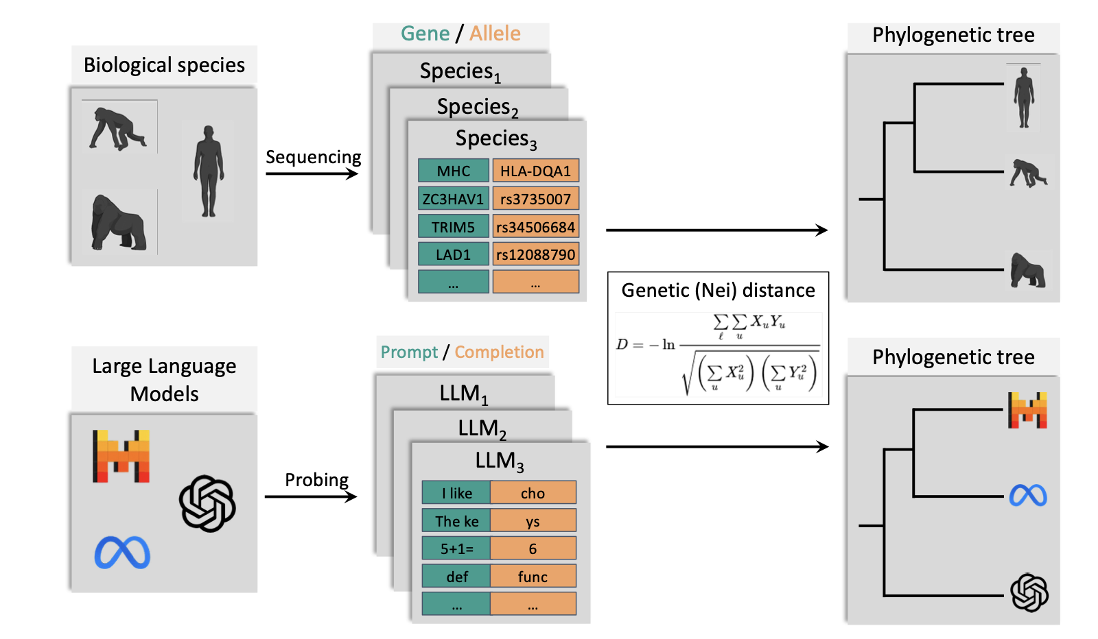 Illustration of the PhyloLM algorithm
This method makes it possible to accurately reconstruct the evolutionary history of LLM families. To illustrate this, we ran an experiment on a family of models for which the ground truth evolutionary tree is known, and used PhyloLM to reconstruct it using only their artificial genetic material — with no prior knowledge of their training history. The result is striking: PhyloLM reconstructs the tree with near-perfect accuracy, as shown below.
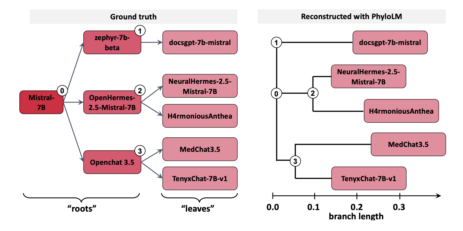 PhyloLM tree reconstruction results
The left panel shows the ground truth and the right panel shows the reconstruction — the two are nearly identical, validating both the analogy and the method.
That said, the reconstructed tree does not include common ancestors. This is standard in biology, where the NJ algorithm is designed to reconstruct relationships between living species whose common ancestors are long extinct and therefore unobservable. In LLMs, however, we have access to all intermediate models — the “ancestors” are not extinct, they are publicly available. This makes the inability to recover common ancestors a meaningful limitation of the current method, and an interesting direction for future work as well as an interesting conceptual observation.
It is also possible to plot a more general dendrogram not taking into account the assumptions of not having common ancestors but also by including several families of models all at once:
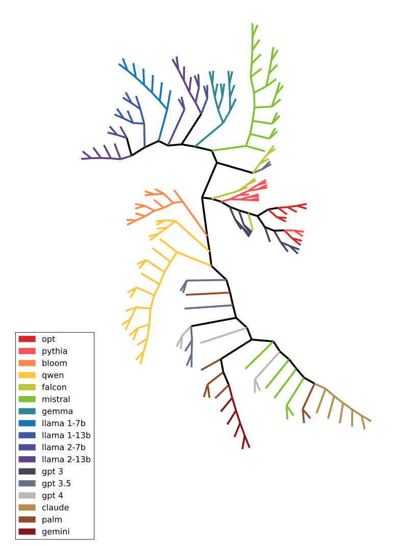
Full dendrogram containing hundreds of LLMs.
This dendrogram is a very nice visualization that, first, PhyloLM is capable of clustering families of models (models finetuned from the same pretrained model show similar behavior) but also that some of these families are similar (like OPT, Pythia and GPT-3) that were likely pretrained on similar training sets. Nonetheless, it is important to remind that the asumptions for using the NJ algorithm are not respected in this context and therefore this cannot be interpreted as an evolutionary tree but rather as a distance visualization tree.
Limitations and open questions
Now that we have seen how PhyloLM works and why the analogy holds, let’s take a step back to recap its assumptions and discuss the limitations and open avenues for future work.
We established that P(token | context) satisfies the three properties identified in Part 2 for a good evolutionary marker: it is universal across all LLMs (if not particularly compressed), it can be made to exhibit moderate variance at the relevant timescale through careful gene selection, and it is the functional grounding of language models by definition. These properties make it well suited to phylogenetic reconstruction — but only under the assumptions that the method relies on.
The most significant of these is the tree-like model of evolution. As we noted in biology, real evolutionary history is closer to a graph than a tree: horizontal gene transfer, convergent evolution, and interbreeding all introduce connections that a tree cannot capture. LLMs face the same issue. Training data shared across model families, distillation — where one model is trained to imitate another — and other forms of cross-lineage influence are all forms of horizontal evolution that the current method does not account for.
There is also a structural difference between biological and artificial evolution that pushes beyond the tree assumption in a deeper way. In biology, it is often considered that all known life shares a single common ancestor: the tree has one root. In LLMs, this concept is more complex. If we consider only vertical inheritance through finetuning, multiple independent roots exist — GPT, Mistral, Llama, and others were each pretrained from scratch by different actors. If we adopt a broader definition of inheritance — encompassing shared neural architectures, training algorithms, and datasets — then a single root becomes more conceivable, perhaps traced back to the original Transformer architecture, but the resulting tree structure becomes far more tangled.
This ambiguity also raises a deeper question about what the tree is actually capturing. Consider two pretrained models A and B, the former finetuned into models C and D with respectively method 1 and 2 and the later in E using method 2. Should C and D be close because they share an ancestor, or should D and E be close because they were finetuned both with method 2 ? PhyloLM captures behavioral similarity without distinguishing between these sources of relatedness, making the interpretation of the resulting tree sometimes less trivial than in biology due to all these horizontal transfers in the evolutionary history of LLMs.
More fundamentally, the flow of genetic information in LLMs is far less constrained than in nature. In biology, populations speciate precisely because contact is lost — genes cannot flow freely between isolated groups. In the LLM ecosystem, training practices, architectures, and datasets circulate freely through scientific papers, open-source releases, and shared benchmarks. This sometimes makes LLM evolution look less like a branching tree and more like a single large population that periodically speciates into new niches (generative AI, chatbots, coding assistants, etc.) as new scientific directions emerge — closer, perhaps, to the evolutionary tree of science than to the traditional tree of life observed in biology.
These observations point to important directions for future work. Current phylogenetic algorithms, designed for the slower and more isolated dynamics of biological evolution, are not well suited to this rapid and highly horizontal form of inheritance. New methods will be needed to handle multiple roots, mixed inheritance signals, and the graph-like structure that better describes how LLMs relate to one another. Additionally, as noted earlier, the NJ algorithm cannot recover common ancestors — a limitation that matters more in LLMs than in biology, since intermediate models remain available and observable. Developing methods that can reconstruct internal nodes, not just leaf relationships, would be a natural and valuable extension.
Ultimately, these limitations are not just obstacles but should be seen as invitations to rethink the field of genetics. They pave the way for a larger sense of genetics, not anchored to biological DNA sequences, but built around general atoms of evolution shared across biological and artificial life forms.
Cite PhyloLM
@inproceedings{ICLR2025_a2e28663,
 author = {Yax, Nicolas and Oudeyer, Pierre-Yves and Palminteri, Stefano},
 booktitle = {International Conference on Learning Representations},
 editor = {Y. Yue and A. Garg and N. Peng and F. Sha and R. Yu},
 pages = {64792--64844},
 title = {PhyloLM: Inferring the Phylogeny of Large Language Models and Predicting their Performances in Benchmarks},
 url = {https://proceedings.iclr.cc/paper_files/paper/2025/file/a2e28663712d5a3429a98918c3058f7b-Paper-Conference.pdf},
 volume = {2025},
 year = {2025}
}
- [1] Dawkins, R. (2006). The Selfish Gene. Oxford University Press.
- [2] d'Huy, J. (2013). A Cosmic Hunt in the Berber sky: a phylogenetic reconstruction of a Palaeolithic mythology. Les Cahiers de l'AARS, 15, pp.93–106.
- [3] Takezaki, N. & Nei, M. (1996). Genetic Distances and Reconstruction of Phylogenetic Trees From Microsatellite DNA. Genetics, 144(1):389–399.
- [4] Saitou, N. & Nei, M. (1987). The neighbor-joining method: a new method for reconstructing phylogenetic trees. Molecular Biology and Evolution, 4(4):406–425.
- [5] Howitz, E. & Kurer, N. & Kahana, J. & Amar, L. & Hoshen, Y. (2025). We Should Chart an Atlas of All the World's Models. ICLR 2025.
- [6] Yax, N. & Oudeyer, PY. & Palminteri, S. (2025). PhyloLM: Inferring the Phylogeny of Large Language Models and Predicting their Performances in Benchmarks. ICLR 2025.
- [7] Momose, O. & Yamagiwa, H. & Takase, Y. & Shimodaira, H. (2025). Mapping 1,000+ Language Models via the Log-Likelihood Vector. ACL 2025.
- [8] Wu, Z. & Zhao, H. & Wang, Z. & Guo, J. & Wang, Q. & He, B. (2026). LLM DNA: Tracing Model Evolution via Functional Representations. ICLR 2026.