Benchmarking#

In this tutorial, we compare simulation times (on CPU on a laptop machine) when simulating models generated with original SBMLtoODEpy library versus with the SBMLtoODEjax library. The code in this notebook is rather complicated, but you can run it on your own machine and customize it to your needs if you want to benchmark for specific SBML models and/or reaction times and/or batch size. Otherwise, we advise jumping directly to the benchmark results which summarizes when (and when not) using SBMLtoODEjax can become advantageous.

Imports and Utils#

Show code cell content Hide code cell content

# imports
import warnings
warnings.filterwarnings("ignore")
warnings.warn("test")

import jax
jax.config.update("jax_platform_name", "cpu")
from jax import vmap
import jax.numpy as jnp
import jax.random as jrandom

import importlib
import os
import time

import matplotlib.pyplot as plt
from multiprocessing import Pool
import numpy as np
from sbmltoodejax.biomodels_api import get_content_for_model
from sbmltoodejax.parse import ParseSBMLFile
from sbmltoodejax.modulegeneration import GenerateModel as GenerateJaxModel
from sbmltoodepy.modulegeneration import GenerateModel as GeneratePyModel


# load model utils
def generate_models(model_idx, deltaT=0.1, atol=1e-6, rtol=1e-12, mxstep=1000):
    
    model_xml_body = get_content_for_model(model_idx)
    model_data = ParseSBMLFile(model_xml_body)
    
    py_model_fp = "py_model.py"
    GeneratePyModel(model_data, py_model_fp)
    
    jax_model_fp = "jax_model.py"
    GenerateJaxModel(model_data, jax_model_fp, deltaT=deltaT, atol=atol, rtol=rtol)
    
    return py_model_fp, jax_model_fp

def load_models(model_idx, deltaT=0.1, atol=1e-6, rtol=1e-12, mxstep=1000):
    # Generate model files
    py_model_fp, jax_model_fp = generate_models(model_idx, deltaT=deltaT, atol=atol, rtol=rtol, mxstep=mxstep)
    
    # Load Jax model
    jax_spec = importlib.util.spec_from_file_location("ModelSpec", jax_model_fp)
    jax_module = importlib.util.module_from_spec(jax_spec)
    jax_spec.loader.exec_module(jax_module)
    
    jax_model_cls = getattr(jax_module, "ModelRollout")
    jax_model = jax_model_cls()
    jax_y0 = getattr(jax_module, "y0")
    jax_w0 = getattr(jax_module, "w0")
    jax_c = getattr(jax_module, "c")
    
    y_indexes = getattr(jax_module, "y_indexes")
    w_indexes = getattr(jax_module, "w_indexes")
    c_indexes = getattr(jax_module, "c_indexes")
    
    
    # Load numpy model
    py_spec = importlib.util.spec_from_file_location("ModelSpec", py_model_fp)
    py_module = importlib.util.module_from_spec(py_spec)
    py_spec.loader.exec_module(py_module)
    
    py_model_cls = getattr(py_module, "SBMLmodel")
    py_model = py_model_cls()
    py_y0, py_w0, py_c = get_sbmltoodepy_model_variables(py_model, y_indexes, w_indexes, c_indexes)


    return (jax_model, jax_y0, jax_w0, jax_c), (py_model, py_y0, py_w0, py_c), (y_indexes, w_indexes, c_indexes)

# utils for converting SBMLtoODEpy according to SBMLtoODEjax conventions (for comparison)
def get_sbmltoodepy_model_variables(model, y_indexes, w_indexes, c_indexes):
    y = np.zeros(len(y_indexes))
    w = np.zeros(len(w_indexes))
    c = np.zeros(len(c_indexes))

    for k, v in model.s.items():
        if k in y_indexes:
            y[y_indexes[k]] = v.amount
        elif k in w_indexes:
            w[w_indexes[k]] = v.amount
        elif k in c_indexes:
            c[c_indexes[k]] = v.amount

    for k, v in model.p.items():
        if k in y_indexes:
            y[y_indexes[k]] = v.value
        elif k in w_indexes:
            w[w_indexes[k]] = v.value
        elif k in c_indexes:
            c[c_indexes[k]] = v.value

    for k, v in model.c.items():
        if k in y_indexes:
            y[y_indexes[k]] = v.size
        elif k in w_indexes:
            w[w_indexes[k]] = v.size
        elif k in c_indexes:
            c[c_indexes[k]] = v.size

    for k, v in model.r.items():
        for sub_k, sub_v in v.p.items():
            if f"{k}_{sub_k}" in w_indexes:
                w[w_indexes[f"{k}_{sub_k}"]] = sub_v.value
            elif f"{k}_{sub_k}" in c_indexes:
                c[c_indexes[f"{k}_{sub_k}"]] = sub_v.value

    return y, w, c


def set_sbmltoodepy_model_variables(model, y, y_indexes):
    """
    Util to set the model variables
    """
    
    for k in model.s.keys():
        if k in y_indexes:
            model.s[k].concentration = y[y_indexes[k]]

    for k in model.p.keys():
        if k in y_indexes:
            model.p[k].value = y[y_indexes[k]]


    for k in model.c.keys():
        if k in y_indexes:
            model.c[k].size = y[y_indexes[k]]

    return model

# plot utils
default_colors = [(204,121,167), 
                  (0,114,178),
                  (230,159,0),  
                  (0,158,115),
                  (127,127,127),
                  (240,228,66),
                  (148,103,189),
                  (86,180,233),
                  (213,94,0),
                  (140,86,75),
                  (214,39,40),
                  (0,0,0)]
default_colors = [tuple([c/255 for c in color]) for color in default_colors]

Run benchmark#

# Simulation for different (rollout durations, number of rollouts in parallel)
all_model_ids = [3, 4, 6, 8, 10]
all_n_secs = [0.1, 1, 10, 100, 1000, 10000, 100000]
all_n_in_parallel = [5, 50, 100, 250, 500, 1000]

# same ODE solver parameters than SBMLtoODEpy ones for fair comparison
deltaT = 0.1
atol = 1e-6
rtol = 1e-12
mxstep = 5000000 

key = jrandom.PRNGKey(0)

# prepare results dictionary
compute_time = {}
compute_time['jax'] = {}
compute_time['py'] = {}
compute_time['py_pool'] = {}
for model_idx in all_model_ids:
    compute_time['jax'][model_idx] = {}
    compute_time['py'][model_idx] = {}
    compute_time['py_pool'][model_idx] = {}
    for n_in_parallel in [1] + all_n_in_parallel: 
        compute_time['jax'][model_idx][n_in_parallel] = {}
        compute_time['py'][model_idx][n_in_parallel] = {}
        compute_time['py_pool'][model_idx][n_in_parallel] = {}


for model_idx in all_model_ids:
    print(f"model_idx: {model_idx}")
    
    # load models
    (jax_model, jax_y0, jax_w0, jax_c), (py_model, py_y0, py_w0, py_c), (y_indexes, w_indexes, c_indexes) = load_models(model_idx, deltaT=deltaT, atol=atol, rtol=rtol, mxstep=mxstep)

    
    # We first test for different n_secs without parallel execution (n_in_parallel = 1)
    n_in_parallel = 1
    for i, n_secs in enumerate(all_n_secs):
        print(f"n_secs: {n_secs}")

        n_steps = int(n_secs / deltaT)


        # Simulate JAX model
        jax_cstart = time.time()
        jax_ys, jax_ws, ts = jax_model(n_steps, jax_y0, jax_w0)
        jax_ys.block_until_ready()
        jax_cend = time.time()

        compute_time['jax'][model_idx][n_in_parallel][n_secs] = jax_cend - jax_cstart

        # Simulate NUMPY model 
        if n_secs <= 1000:

            py_cstart = time.time()
            for step_idx in range(n_steps):
                py_model.RunSimulation(deltaT, absoluteTolerance=atol, relativeTolerance=rtol)
            py_cend = time.time()

            compute_time['py'][model_idx][n_in_parallel][n_secs] = py_cend - py_cstart
        
        else:
            # we do linear approximation for big n_secs (too long to run)
            prev_n_secs = all_n_secs[i-1]
            ratio = n_secs/prev_n_secs
            compute_time['py'][model_idx][n_in_parallel][n_secs] = compute_time['py'][model_idx][n_in_parallel][prev_n_secs]*ratio
        
        
    # We then test different number of simulations launched in parallel and n_secs = 10
    n_secs = 10
    n_steps = int(n_secs / deltaT)
    
    # batch jax model
    batched_jax_model = vmap(jax_model, in_axes=(None, 0, 0), out_axes=(0, 0, None))
    
    # Create batched init (by adding perturbation to default init state)
    key, subkey = jrandom.split(key)
    perturb = jrandom.uniform(subkey, (all_n_in_parallel[-1], len(jax_y0)), minval=0.0, maxval=5.0)
    batched_jax_y0 = jnp.maximum(jnp.tile(jax_y0, (all_n_in_parallel[-1], 1)) + perturb, 0.0)
    batched_jax_w0 = jnp.tile(jax_w0, (all_n_in_parallel[-1], 1))
    batched_py_y0 = np.array(batched_jax_y0)
    
    for i, n_in_parallel in enumerate(all_n_in_parallel):
        print(f"n_in_parallel: {n_in_parallel}")
    
        # Simulate JAX model
        jax_cstart = time.time()
        jax_ys, jax_ws, ts = batched_jax_model(n_steps, batched_jax_y0[:n_in_parallel], batched_jax_w0[:n_in_parallel])
        jax_ys.block_until_ready()
        jax_cend = time.time()
        
        compute_time['jax'][model_idx][n_in_parallel][n_secs] = jax_cend - jax_cstart
        
        # Simulate NUMPY model with for loop over init states
        if n_in_parallel <= 100:
        
            py_ctime = 0
            for cur_py_y0 in batched_py_y0[:n_in_parallel]:

                # Change initial state 
                py_model = set_sbmltoodepy_model_variables(py_model, cur_py_y0, y_indexes)

                # Run simulation
                py_cstart = time.time()
                for step_idx in range(n_steps):
                    py_model.RunSimulation(deltaT, absoluteTolerance=atol, relativeTolerance=rtol)
                py_cend = time.time()

                py_ctime += py_cend - py_cstart

            compute_time['py'][model_idx][n_in_parallel][n_secs] = py_ctime
        
        else:
            # we do linear approximation for big n_in_parallel (too long to run)
            prev_n_in_parallel = all_n_in_parallel[i-1]
            ratio = n_in_parallel/prev_n_in_parallel
            compute_time['py'][model_idx][n_in_parallel][n_secs] = compute_time['py'][model_idx][prev_n_in_parallel][n_secs]*ratio
        
        
        # Simulate NUMPY model with pooling over init states
        def simulate_py_model(cur_py_y0):
            # Change initial state 
            cur_py_model = set_sbmltoodepy_model_variables(py_model, cur_py_y0, y_indexes)

            # Run simulation
            for step_idx in range(n_steps):
                cur_py_model.RunSimulation(deltaT, absoluteTolerance=atol, relativeTolerance=rtol)

            return

        # Simulate the OOP Numpy/Scipy-based Model
        py_cstart = time.time()
        p = Pool()
        res = p.map(simulate_py_model, [cur_py_y0 for cur_py_y0 in batched_py_y0[:n_in_parallel]])
        py_cend = time.time()
        
        compute_time['py_pool'][model_idx][n_in_parallel][n_secs] = py_cend - py_cstart

Benchmark results#

../_images/e1d11cba84f2799fb40bf8d885a294f6aa76bddc25ed85ef445ec23e65d7ce9a.png

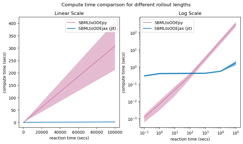
Above we show the average compute time of model rollouts for different rollout lengths (reaction times), for models generated with the original SBMLtoODEpy library (shown in pink) versus with the SBMLtoODEjax library (shown in blue).

We can see that for short reaction times (here <100 secs with \(\Delta T=0.1\), see Log Scale), SBMLtoODEjax simulation takes longer than the original SBMLtoODEpy library because when calling ModelStep for the first time, it takes some time to generate the compiled trace. However, the advantage of SBMLtoODEjax becomes clear when considering longer rollouts where we obtain huge speed-ups with respect to original SBMLtoODEpy library (see Linear Scale). This is because the original SBMLtoODEpy python code uses for-loops, hence have linear increase of compute time, whereas the scanned JIT-compiled step function executes much faster.

../_images/acead121cf06dc2007d6584afcf9077f331ebc0b63657b0ee3fe618b740160fe.png

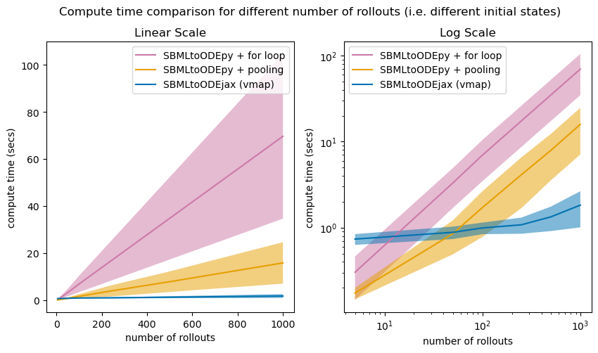
Above we show the average compute time of model rollouts for different batch sizes (x-axis), where all runs have a rollout length of 10 seconds with \(\Delta T=0.1\). We compare the average compute time of model rollouts for 1) the SBMLtoODEpy-generated models and for loop computations over the inputs (pink), 2) the SBMLtoODEpy-generated models and pooling over the inputs (orange) and 3) the SBMLtoODEjax library with vectorized computations (blue).

Again, similar conclusions can be drawn where SBMLtoODEjax is less efficient for small batch sizes (and small rollout lengths), but becomes very advantageous for larger batch sizes.

⚠️ Benchmark limitations#

Our benchmark only compares with the SBMLtoODEpy library, as we directly extend from it, which relies on the Numpy/Scipy backend. Other software tools, such as Tellurium which relies on the C++ libRoadRunner backend, might be more performant.
Whereas we use similar hyper-parameters for the ODE equation solvers (absolute and relative tolerance and maximum number of solver steps), SBMLtoODEpy uses scipy.integrate.odeint solver whereas SBMLtoODEjax uses jax.experimental.odeint solver, which might have some impact on the precision of the results and would need to be more rigorously examined as well argued in this paper.

Benchmarking

Contents

Benchmarking#

Imports and Utils#

Run benchmark#

Benchmark results#

⚠️ Benchmark limitations#