Parallel execution

In this tutorial, we will see how to efficiently run simulations of the model for a batch of different initial conditions, in a vectorized manner using JAX vmap transformation. We will use it to visualize, in phase space, the trajectories of this SBML model starting from a grid of different initial conditions. As you will see, vectorizing the model will require only few lines of code.

Imports and Utils

Show code cell content Hide code cell content

import importlib
from itertools import combinations

import jax
jax.config.update("jax_platform_name", "cpu")
import jax.numpy as jnp
from jax import vmap

import matplotlib.pylab as plt
from matplotlib.colors import hsv_to_rgb
from matplotlib.transforms import Affine2D, offset_copy
from sbmltoodejax.utils import load_biomodel

Show code cell content Hide code cell content

# Plot Utils
default_colors = [(204,121,167), 
                  (0,114,178),
                  (230,159,0),  
                  (0,158,115),
                  (127,127,127),
                  (240,228,66),
                  (148,103,189),
                  (86,180,233),
                  (213,94,0),
                  (140,86,75),
                  (214,39,40),
                  (0,0,0)]
default_colors = [tuple([c/255 for c in color]) for color in default_colors]

def plot_time_trajectory(ts, ys, y_indexes):
    plt.figure(figsize=(6, 4))
    for y_label, y_idx in y_indexes.items():
        plt.plot(ts, ys[y_idx, :], color=default_colors[y_idx], label=y_label)
    plt.legend()
    plt.show()
    
def plot_phase_space_trajectories(ys, y_indexes, plot_every=1):

    fig = plt.figure(figsize=(7,7))
    ax = fig.add_subplot(projection='3d')
    
    # plot trajectories
    X = ys[..., 0, :-1][..., ::plot_every]
    Y = ys[..., 1, :-1][..., ::plot_every]
    Z = ys[..., 2, :-1][..., ::plot_every]
    U = ys[..., 0, 1:][..., ::plot_every] - X
    V = ys[..., 1, 1:][..., ::plot_every] - Y
    W = ys[..., 2, 1:][..., ::plot_every] - Z
    
    T = X.shape[-1]
    if X.ndim == 2:
        batch_size = X.shape[0]
    else:
        batch_size = 1
    c = ([hsv_to_rgb((step / (2*T), 1, 1)) for step in range(T)][::plot_every])*batch_size
    ax.quiver(X.flatten(), Y.flatten(), Z.flatten(), 
              U.flatten(), V.flatten(), W.flatten(), 
              color=c, arrow_length_ratio=0)
    
    # plot starting points
    ax.scatter(ys[..., 0, 0], ys[..., 1, 0], ys[..., 2, 0], color="red")

    for y_name, y_idx in y_indexes.items():
        if y_idx == 0:
            ax.set_xlabel(y_name)
        elif y_idx == 1:
            ax.set_ylabel(y_name)
        elif y_idx == 2:
            ax.set_zlabel(y_name)
    plt.show()

Running the default trajectory in phase space

# Load model
model_idx = 156
model, default_y0, default_w0, default_c = load_biomodel(model_idx)

# Run simulation
n_secs = 100
n_steps = int(n_secs / model.deltaT)
default_ys, default_ws, ts = model(n_steps)

# Plot time-course evolution and corresponding trajectories in phase space
plot_time_trajectory(ts, default_ys, model.modelstepfunc.y_indexes)
plot_phase_space_trajectories(default_ys, model.modelstepfunc.y_indexes)

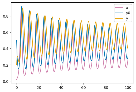
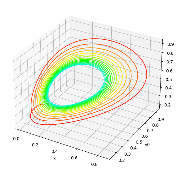
The model only has 3 nodes \((x, y0, y)\). Top plot shows the time-course evolution of the node states over time, and bottom plot shows the same trajectory in phase space. Here the trajectory starts from the default initial conditions provided in the original SBML file: \((x=0.02, y0=0.5, y=0.2)\). Colorscale in phase-space displays time evolution from t=0 (red) to t=100 secs (cyan).

Running simulation in batch mode, for a grid of different starting conditions

This time we want to run the model starting from a grid of 4x4x4 initial conditions. Let’s start by creating a batched_y0 vector that contains the different starting points (flatten grid of initial conditions).

# batch y0 
r=5
ymin = 1/r * default_ys.min(-1)
ymax = r * default_ys.max(-1)
n_inits_per_dim = 4
grid = jnp.meshgrid(
    *[
        jnp.linspace(ymin[node_idx], ymax[node_idx], n_inits_per_dim)
        for node_idx in range(len(ymin))
    ]
)
batched_y0 = jnp.stack([dim_grid.flatten() for dim_grid in grid], axis=-1)

Then, to run the model in a vectorized manner from this batch of initial conditions, one simply needs to vectorize the model function with JAX vmap transformation, and then calling this vectorized function in the exact same way as before:

# batch model
batched_model = vmap(model, in_axes=(None, 0), out_axes=(0, 0, None))

# run simulation in batch mode
batched_ys, batched_ws, ts = batched_model(n_steps, batched_y0)

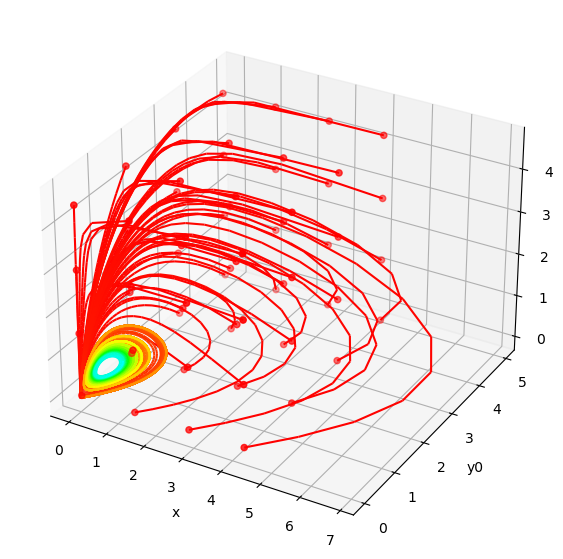
We can then run the resulting trajectories in phase space to observe the behaviors. Here we can see that all trajectories converge to the same orbit, despite starting from different positions.

plot_phase_space_trajectories(batched_ys, model.modelstepfunc.y_indexes)